Three detailed fluctuation theorem
Three detailed fluctuation theorem
Recap the fluctuation theorems
Weak system-resevoir coupling
Crooks relation \(\frac{P(W)}{\bar{P}(-W)}=\exp\left[\beta(W-\Delta F)\right]\)
Jaryzynski equality
\[\langle \exp(-\beta W)\rangle =\exp(-\beta \Delta F)\]More general case
detailed and integral fluctuation theorem
For a random variable $R$ it satisfy integral fluctuation theorem if
\[\langle e^R\rangle=1\]and the detailed fluctuation theorem
\[\exist\bar{P}\quad \frac{P(R)}{\bar{P}(-R)}=e^{R}\quad\forall R\]Relative entropy/Kullback-Leibler distance
Kullback-Leibler distance characterize the difference between two probability distribution, for a set of random variable(s) $\mathbf{m}$ and two probability distribution $P \(\mathcal{D}(P||\mathcal{\tilde{P}})=\sum_mP_\mathbf{m}\ln\frac{P_\mathbf{m}}{\tilde{P}_\mathbf{m}}\)
For single trajectory, the distance between two trajectory is defined as
\[r_\mathbf{m}=\ln\frac{P_\mathbf{m}}{\tilde{P}_\mathbf{m}}\]One can verify that the random variable $r_\mathbf{m}$ satisfy fluctuation theorem
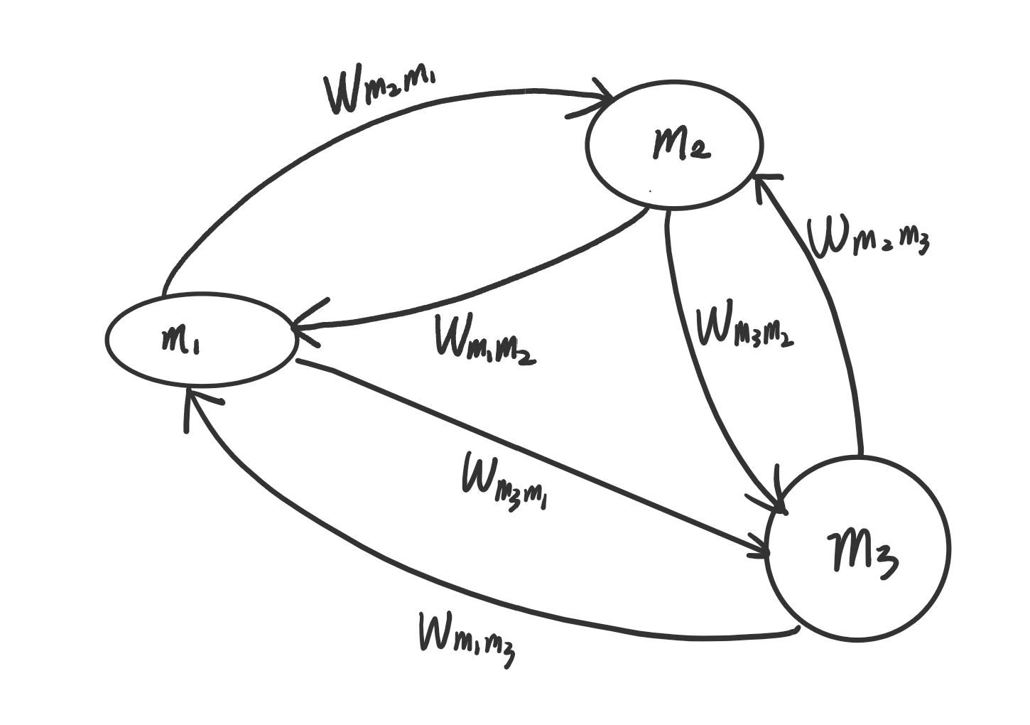
A physical system characterized by master equation
Master equation \(\dot{p}_m(t)=\sum_{m'}W_{m.m'}(\lambda_t)p_{m'}(t)\)

Probability of tranjectory
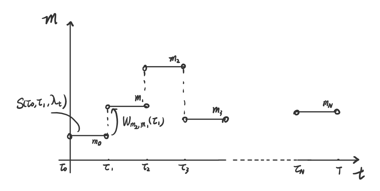
Now suppose we have a trajectory $\mathbf{m}={m_t,t\in [0,T]}$, discretized the time into $N$ steps, we can write down the probability of hte trajectory explicitly 
where $S_{m_{j-1}}(\tau_{j-1},\tau_j)$ is the survival probability
\[S_{m_{j-1}}(\tau_{j-1},\tau_j,\lambda_\tau)=\exp\left[\int_{\tau_{j-1}}^{\tau_j}d\tau'\ W_{m_{j-1},m_{j-1}}(\lambda_{\tau'})\right]\]we can also write down the probability of the reversed process
\[\bar{\lambda}_t=\lambda_{T-t},\ \bar{m}_j=m_{N-j}\] \[\begin{aligned} \bar{P}_{\bar{m}} &=\prod_{j=0}^Np_{\bar{m}_{j}}(\tau_{j},\tau_{j+1})\\ &=p_{m_N}(T)\left[\prod_{j=1}^N S_{m_j,m_j}(\tau_{j+1},\tau_j,\bar{\lambda}_{T-\tau})W_{m_{j-1},m_j}\right]S_{m_0}(\tau,0,\bar{\lambda}_{T-\tau}) \end{aligned}\]Total entroy production
\[\Delta S_{tot}[\mathbf{m}]\equiv \ln\frac{P_{\mathbf{m}}}{\bar{P}_\mathbf{\bar{m}}}\]system+reservoir picture
\[\Delta S_{tot}[\mathbf{m}]=\underbrace{\ln\frac{p_{m_0}(0)}{p_{m_N}(T)}}_{\text{system entropy}}+\underbrace{\sum_{j=1}^N\ln\frac{W_{m_j,m_{j-1}}(\lambda_{\tau_j})}{W_{m_{j-1},m_j}(\lambda_{\tau_j})}}_{\text{reservoir entropy}}\]adiabatic+non-adiabatic picture
Using the steady state distribution $p_m^{st}(\lambda_t)$ \(\sum_{m'}W_{m,m'}(\lambda_t)p_m^{st}(\lambda_t)=0\)
we can split total entropy production to two parts, the adiabatic entropy production and the non-adiabatic entropy production
\[\Delta S_{tot}[\mathbf{m}]=\underbrace{\ln\frac{p_{m_0}(0)}{p_{m_N}(T)}+\sum_{j=1}^N\ln\frac{p_{m_j}^{st}(\lambda_{\tau_j})}{p_{m_{j-1}}^{st}(\lambda_{\tau_j})}}_{\text{adiabatic }\Delta S_a[\mathbf{m}]} +\underbrace{\sum_{j=1}^N\ln\frac{W_{m_j,m_{j-1}}(\lambda_{\tau_j})p_{m_{j-1}}^{st}(\lambda_{\tau_j})}{W_{m_{j-1},m_{j}}(\lambda_{\tau_j})p_{m_{j}}^{st}(\lambda_{\tau_j})}}_{\text{non-adiabatic }\Delta S_{na}[\mathbf{m}]}\]If the system’s steady state satisfy detailed balance condition \(W_{m,m'}(\lambda_t)p_{m'}^{st}(\lambda_t)=W_{m',m}(\lambda_t)p_m^{st}(\lambda_t)\quad\forall m,m'\) the adbiatic contribution is zero \(\Delta S_a[\mathbf{m}]=0\)
If the relaxiation process is much faster than the time scale of $\lambda_t$ \(\langle\Delta S_{na}[\mathbf{m}]\rangle=0\)
Three fluctuation theorems
By introducing the adjoint transition matrix $\mathbf{W}^+$
\[W_{m,m'}^+=\frac{W_{m',m}(\lambda_t)p_m^{st}(\lambda_t)}{p_{m'}^{st}(\lambda_t)}\]one can obtain the following relation
\[\Delta S_{na}[\mathbf{m}]\equiv\ln\frac{P_\mathbf{m}}{\bar{P}_{\mathbf{\bar{m}}}^+},\quad \Delta S_a[\mathbf{m}]\equiv\frac{P_{\mathcal{m}}}{P_{\mathbf{m}}^+}\]Using the mathematical relation we introduced before, one can obtain three detailed fluctuation theorems
\(\frac{P(\Delta S_{tot})}{\bar{P}(-\Delta S_{tot})}=e^{\Delta S_{tot}}\) \(\frac{P(\Delta S_{na})}{\bar{P}^+(-\Delta S_{na})}=e^{\Delta S_{na}},\quad \frac{P(\Delta S_{a})}{P^+(-\Delta S_{a})}=e^{\Delta S_{a}}\)
