Jekyll2024-07-20T23:43:48-07:00https://shiling42.github.io/feed.xmlShiling Liang PhD student in Physics@LBS, EPFLShiling Liang 梁师翎shiling.liang@epfl.chCoding with GPT-4: Simulating Emergent Phenomena in Complex Systems2023-03-21T00:00:00-07:002023-03-21T00:00:00-07:00https://shiling42.github.io/posts/2023/03/GPT-simulator
This article was generated by GPT-4 under guidance.
Introduction
Today we bring you a unique online interactive physics system simulation project, which uses HTML and JavaScript code generated by GPT-4 to implement a series of visual simulations that allow us to better understand physics, complex systems, and emergent phenomena.
In this project, we will show you some exciting simulations, including the XY model, the Vicsek bird flocking model, phase separation, and particle repulsion. These simulations all use code generated by GPT-4, allowing us to explore the physical world intuitively and understand various physical processes and emergent phenomena.
In addition, with the help of GPT-4, the natural language processing tool, programming becomes simpler, allowing more people to participate in project development. Even people without interface development experience can quickly develop such projects by commanding GPT-4 in ordinary language.
In this project, we will guide you through how to use GPT-4 technology to generate code for interactive physics system simulations, allowing you to experience the charm of physics and complex systems. Let’s start this exploration journey together!
Today, we are excited to introduce a cutting-edge, online interactive physics system simulation project that leverages the power of GPT-4-generated HTML and JavaScript code to create a suite of visually engaging simulations, aimed at enhancing our understanding of physics, complex systems, and emergent phenomena.
In this project, we showcase captivating simulations such as the XY model, the Vicsek bird flocking model, phase separation, and particle repulsion. Each of these simulations is powered by code generated by GPT-4, enabling us to explore the physical world in an intuitive manner and gain insights into various physical processes and emergent phenomena.
Furthermore, GPT-4’s natural language processing capabilities simplify the programming process, making it more accessible for a wider audience to contribute to the project’s development. Individuals without prior experience in interface development can swiftly create projects by providing GPT-4 with plain-language instructions.
Throughout this project, we will walk you through the process of utilizing GPT-4 technology to generate code for interactive physics system simulations, offering you the opportunity to delve into the fascinating world of physics and complex systems. Let’s embark on this thrilling journey of exploration together!
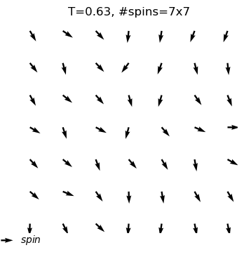
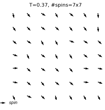
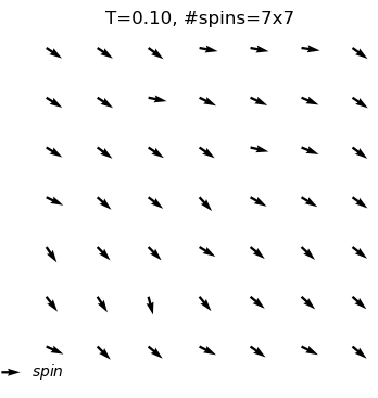
The XY model originates from condensed matter physics and mainly studies a particle system on a two-dimensional plane. These particles can be imagined as compasses, distributed on the plane, and each particle has a direction. The core of this model lies in the interaction between particles: each particle tends to maintain the same direction as neighboring particles. This interaction forms an interesting balance, where particles strive to maintain consistency while responding to the influence of other particles.
In the XY model, we can observe a fascinating emergent phenomenon: when the interaction between particles reaches a certain degree, the entire system will spontaneously form an ordered state, and the particles will point in roughly the same direction. This ordered state reflects the self-organizing behavior inside the system and is a typical phenomenon in complex systems.
The XY model also contains a very interesting and important physical phenomenon - the Berezinskii–Kosterlitz–Thouless (BKT) phase transition. The discovery of the KT phase transition brought revolutionary breakthroughs to the theory of phase transitions, and even led to the Nobel Prize in Physics being awarded to physicists Kosterlitz and Thouless in 2016.
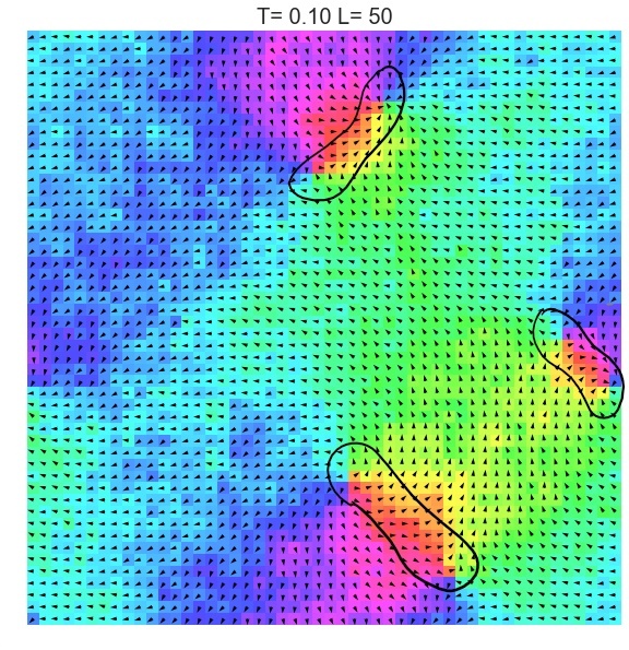
Unlike the first- and second-order phase transitions we are familiar with, such as water turning into ice or water vapor, the KT phase transition is a topological phase transition. This means that it does not involve a sudden change in the density, magnetism, or other physical properties of matter, but rather involves a change in the internal topological structure of the system. In the XY model, this topological structure is manifested as vortices and antivortices, which can be understood as local rotational structures with different rotation directions.
When the temperature is low, vortices and antivortices form a stable paired state, and their mutual attraction makes the system present an ordered state. However, when the temperature rises to a critical point, vortices and antivortices begin to dissociate, and the degree of order in the system gradually decreases. This is the process described by the KT phase transition.
Through the XY model in the online interactive physics system simulation project, we can intuitively observe the process of the KT phase transition and understand how this unique topological phase transition occurs in complex systems. This is undoubtedly an attractive learning path for science enthusiasts who want to deepen their understanding of phase transitions, topological structures, and emergent phenomena.
Phase separation is a widely existing phenomenon in nature, which refers to the spontaneous separation of different types of components into regions of a single component in a mixed system under certain conditions. This process is involved in many chemical, physical, and biological systems, such as oil-water mixtures, cooling and separation of alloys, and distribution of lipid molecules on cell membranes.
The concept closely related to phase separation is pattern formation, which describes the self-organizing phenomenon of spatial structure under certain conditions. This phenomenon is often accompanied by the appearance of local structure and order. In the process of phase separation, we can observe a series of complex pattern formation phenomena, such as bubble-like structures, stripe-like structures, etc. These patterns can be understood as stable structures formed by the system in the process of trying to reduce energy.
In the online interactive physics system simulation project, the phase separation model uses a simplified two-dimensional particle system to simulate the phase separation phenomenon. Although this model is simplified, it can intuitively demonstrate the basic mechanisms of phase separation, such as like attraction, unlike repulsion, and random motion between particles.
In this ChatGPT-assisted project website, we strive to present an engaging and educational online physics visualization platform. Through this platform, users can personally interact with a variety of physical phenomena and complex systems, gaining a more intuitive and vivid understanding of the principles underlying these phenomena.
Our project website features multiple physics simulation examples generated by GPT-4, such as the Vicsek model, the XY model, and the phase separation model. These models are designed to help users comprehend the operational principles and emergent phenomena of complex systems. Additionally, the website offers a series of mouse-interactive models, enabling users to experience the allure of physical phenomena through real-time interaction.
Coding with GPT-4
To conclude this article, let’s discuss how this project was brought to life through ChatGPT. In implementing the phase separation project, I didn’t specify any particular model. Instead, I provided the following requirements:
Implement a visual phase separation model using HTML.
Add repulsion to the model to prevent particle aggregation.
Handle boundary conditions.
Introduce temperature as a parameter.
Add sliders to control all parameters.
Based on these requirements, ChatGPT generated the corresponding HTML and JavaScript code, creating an interactive physics simulation project (there were five or six conversations from the initial command to the generation of a functional model that could display phenomena, followed by more detailed discussions with ChatGPT to refine the page’s appearance). Throughout this process, GPT-4 exhibited an incredible ability to understand my project’s core objectives based on my requirements and generate the appropriate code to fulfill them. It is worth noting, however, that there is a limit to the length of code output by ChatGPT. If the output is interrupted, you can copy and paste the end of the output code and ask GPT to continue writing, ensuring a seamless code-writing process.
Although I’m not well-versed in JavaScript syntax details, I was able to understand how specific calculations were implemented in the physics portion by examining the code (as a pseudo-code reader), which allowed me to verify its accuracy. Overall, correctness checks still require some coding experience, but developers don’t need to know every syntax detail.
For the interface layer, the logic is visually apparent, so it can also be checked. If errors are detected, feedback can be given directly, and GPT-4 possesses a robust self-checking capability.
In collaboration with ChatGPT, we have successfully developed a fun and practical online interactive physics system simulation project. This project not only enables us to grasp complex physical phenomena intuitively but also showcases GPT-4’s enormous potential in code generation and project implementation. Furthermore, GPT-4’s powerful features have saved significant time and effort during the development process, making it possible for physicists and novices alike to swiftly create high-quality visualization and interactive projects.
In conclusion, while GPT-4 cannot currently replace all human work, it can significantly streamline the development process and empower beginners to accomplish tasks that were previously unattainable. In the future, we eagerly anticipate deeper collaboration with artificial intelligence technologies like GPT-4 to explore more innovative applications and solutions.
]]>Shiling Liang 梁师翎shiling.liang@epfl.chThermophroesis as an emergent phenomenon: the role of internal states2023-01-02T00:00:00-08:002023-01-02T00:00:00-08:00https://shiling42.github.io/posts/2023/01/Thermophoresis
In our recent paper, we showed that thermophoresis can be an emergent phenomenon from chemical reaction systems. This blog is a lay summary of our work.
What is thermophoresis?
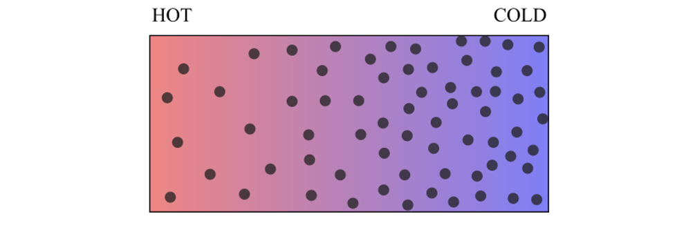
After establishing a temperature gradient in a solution system, we may observe the accumulation of solute particles on the cold or warm side. This phenomenon is known as thermophoresis. Its exact microscopic origin is still under debate. In our work1, we propose a simple and intuitive mechanism to explain this phenomenon, which relies on the correlation of the energy-diffusion properties of the different states of the particles. It is based on a simple idea: particles stay longer where diffusion is slower, and temperature can modulate the transport property of particles.
The phenomenon of inhomogeneous concentration gradients driven by a temperature gradient.
From Einstein’s diffusion relation to thermophoresis
For the understanding of thermophoresis we can go back to the basic Einstein relation of diffusion:
\[D= \frac{T}{\gamma}\propto T R^{-1}\]
The diffusion coefficient is proportional to the temperature divided by the damping constant, and the larger the particle the greater the damping (damping is proportional to particle size), which leads to an inverse relationship between diffusion coefficient and particle size as shown above.
Why do we mention the diffusion coefficient? Because the thermophoretic mechanism we propose here is rooted in nonhomogeneous diffusion and is simply based on a simple concept:
Particles tend to stay in the slow diffusion region for a longer time
This is quite intuitive idea. The diffusion process is essentially the random walk of microscopic particles, and where the random walk is slow, the particles will wander around for a longer time.
Then the emergence of thermophoresis is natural: the diffusion coefficient depends on temperature. Therefore, let’s look at the first term of Einstein’s relation, $\boxed{T}R^{-1}$. Isn’t it exactly the temperature? To put it more bluntly, this term tells us that particles diffuse faster in hot places and slower in cold places.
The temperature term in Einstein’s relation gives us a direct Soret coefficient:
\[S_T^0=\frac{1}{T}\]
However, there are two issues with this simple result.
This coefficient is always positive, which means that it can only indicate the tendency of accumulation in the cold region, namely the thermophoretic phenomenon. In contrast, it is observed experimentally that solute particles can move to the hot region.
This Soret coefficient is two orders of magnitude smaller than the experimentally measured values.
So we need to extract additional information from the Einstein relation. If we look at the Einstein relation again, $D\propto T R^{-1}$, there is a term related to the size of the particle, so can we derive thermophoresis from this term? The answer is yes, and this is the focus of our paper: chemical thermophoresis.
Chemical thermophoresis
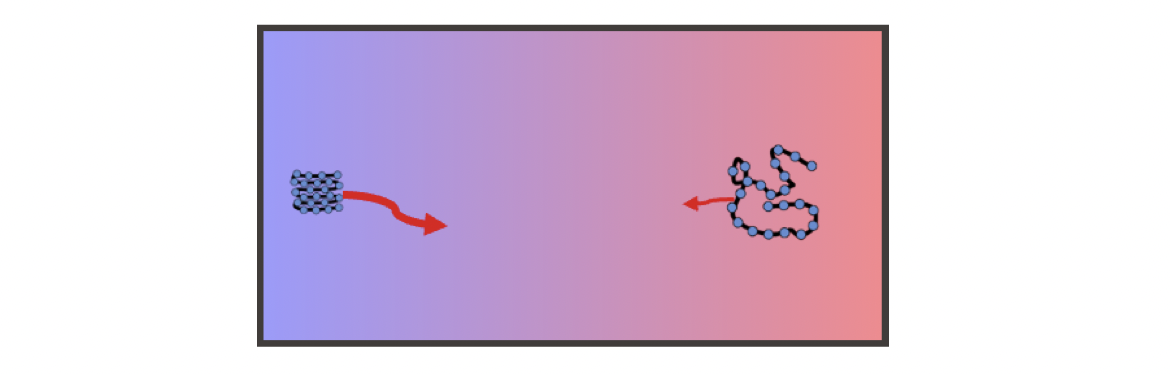
To understand the thermophoresis from thermoresponsive particle size, we can start with a simple and intuitive example which is the foldable polymer
Folded and unfolded states of a polymer.
A polymer can be in both folded and unfolded states. These two states have different free energies, taking into account the interactions between the various parts of the long chain and the interaction with the solvent molecules. Also, it is straightforward that the unfolded state of the polymer has a larger size. The Einstein relation tells us that particles of larger size encounter greater damping and diffuse more slowly. So, if temperature regulates the switching between these two states, we immediately have an average size that depends on temperature and thus a temperature-dependent effective diffusion coefficient.
And this temperature regulation is obvious, especially if we consider that the switching between unfolding and folding is reached fast enough in comparison to diffusion, the probability of being in each state is determined by the local temperature (local equilibrium approximation).
\[p_i=\frac{1}{Z}e^{-G_i/k_BT(x)}\]
From the above Boltzmann distribution, which is the most fundamental law in thermodynamics, we can see that the probability of being in each state depends on the free energy of the state and the temperature of the local environment. Then, if we calculate the average, the effective diffusion coefficient is
\[\langle D\rangle = p_u D_u +p_fD_f\]
which directly depends on the occupations in the two states, and the occupations are determined by the local temperature. Therefore, we have an effective diffusion coefficient that depends on the temperature.
To gain a better understanding, let’s consider the following limit: in the cold region, the particle is almost completely in the folded state, while in the hot region it is almost completely unfolded. The unfolded state in the hot region diffuses more slowly and thus leads to a negative Soret coefficient, which means that such a polymer can show thermophilic behavior.
Polymer can show thermophilic behavior.
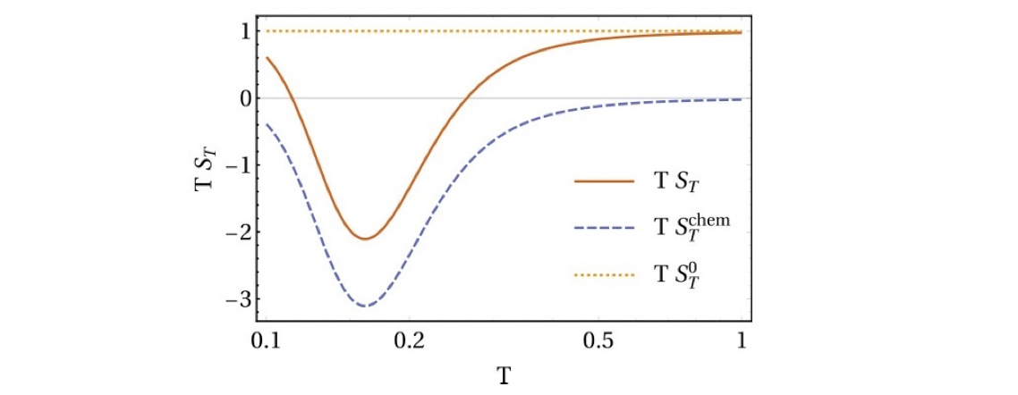
Of course, in the limit case shown above, the always positive term, $S_T^0=1/T$, is not included. Overall, the thermophoresis of the particle depends on $D\propto \boxed{T}\boxed{R^{-1}}$ these two individual contributions. In the case of the example polymer, these two terms are positive and negative, respectively, which leads to the fact that the particle can switch from thermophobic to thermophilic as the temperature changes, i.e. the sign of the Soret coefficient changes. This positive and negative thermophoresis of polymers has been widely observed in experiments2.
The thermotropic and thermophilic behaviors of polymer be changed depending on the temperature.
Here $S_T^0=1/T$ is the contribution of the direct temperature-dependent term. While $S_T^\mathrm{chem}$ is what we call chemical thermophoresis, which originates from the thermoresponsive particle size.
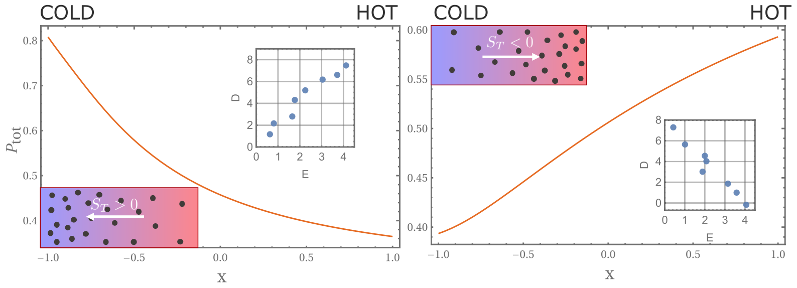
For a more general case, we can consider that the particles have many internal states, which have different energies and diffusion coefficients. This energy-diffusion correlation leads to chemical thermophoresis. We can derive a very simple expression for the chemical Soret coefficient as
Here, the Soret coefficient is directly related to the covariance between the energies and the diffusion coefficients. If the energy and diffusion coefficients of the different states are positively correlated, we get a positive Soret coefficient, i.e. thermophobic, and vice versa, a more interesting thermophilic behavior.
Positive or negative chemical thermophoresis depends on the energy-diffusion correlation.
Complex chemical reactions
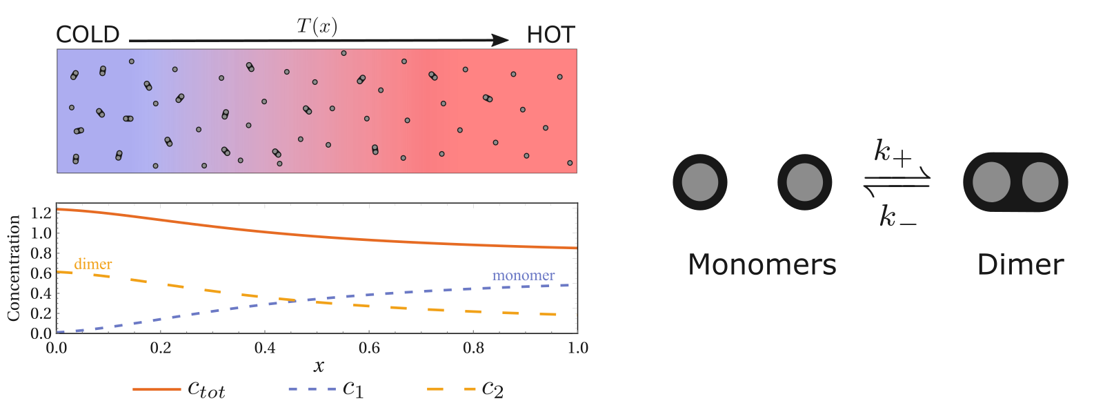
The chemical reactions covered in the previous section are the basic isomerization reactions, that is, no chemical complexes are formed. However, conceptually, it is straightforward to extend the chemical thermophoresis to more complex chemical reactions. For example, the following polymerization reaction
Dimerization reaction can also exhibit thermophoresis.
Two monomers can form a dimer. Although the Soret coefficient derived from the previous isomerization cannot be directly applied, we can still use the energy-diffusion coefficient correlation to understand this thermophoretic phenomenon. Here, the energy and diffusion coefficients of the monomer and dimer are different, and as long as they are not the same, the system can respond to the temperature gradient and exhibit thermophoresis (inhomogeneous distribution) of the total concentration.
Discussion
Our theory gives a microscopic mechanism for the emergence of thermophoresis, which can be decomposed into several terms: the contribution of the temperature term of the Einstein relation itself, and the chemical thermophoresis as a consequence of energy-diffusion correlation. The actual thermophoretic phenomenon might be influenced by other mechanisms, such as those originating from the direct interaction of the particles with the solvent molecules34. Therefore, the emergent chemical thermophoresis we discuss here may be the dominant term, but it may also be a small higher-order quantity that can be neglected. From our understanding, it is highly likely to observe chemical thermophoresis as the dominant mechanism when the structure of the particle is very sensitive to temperature change. For example, in PNIPAM systems, the folding and unfolding of the polymer exhibit phase transition with temperature, and “giant thermophoresis” can be measured at this phase transition point567. We expect that some experiments will be inspired to explore this direction.
Liang S, Busiello D M and De Los Rios P, 2022. Emergent thermophoretic behavior in chemical reaction systems. New Journal of Physics 24 123006↩
Wang Z, Kriegs H and Wiegand S 2012 Thermal diffusion of nucleotides J. Phys. Chem. B 116 7463–9↩
Burelbach Jerome, Frenkel D, Pagonabarraga I and Eiser E 2018 A unified description of colloidal thermophoresis Eur. Phys. J. E 41 1–12↩
Piazza R 2008 Thermophoresis: moving particles with thermal gradients Soft Matter 4 1740–4↩
Kita R and Wiegand S 2005 Soret coefficient of poly (n-isopropylacrylamide)/water in the vicinity of coil- globule transition temperature Macromolecules 38 4554–6↩
Wongsuwarn S, Vigolo D, Cerbino R, Howe A M, Vailati A, Piazza R and Cicuta P 2012 Giant thermophoresis of poly(n-isopropylacrylamide) microgel particles Soft Matter 8 5857–63↩
Königer A, Plack N, Köhler W, Siebenbürger M and Ballauff M 2013 Thermophoresis of thermoresponsive polystyrene–poly (n-isopropylacrylamide) core–shell particles Soft Matter 9 1418–21↩
]]>Shiling Liang 梁师翎shiling.liang@epfl.chNotes on Fluctuation Theorems2018-11-14T00:00:00-08:002018-11-14T00:00:00-08:00https://shiling42.github.io/posts/2018/11/Notes-on-Fluctuation-TheoremsGet the PDF
Abstract
These notes are based on the review article by E.M Sevick et al[1]. on the fluctuation theorem. I also refer to the original papers of Jarzynski[2-4] and adopt notation from a book written by Evans et al.[5]. I discuss the motivation for proposing the fluctuation theorem and provide a detailed derivation of the Evans-Searles Fluctuation Theorem, which shows how macroscopic irreversibility emerged from the time-symmetrical equation of motion and addresses the importance of the initial condition of the system. I also recap the derivation the Crooks Fluctuation Theorem to relate work and free energy of a non-quasistatic process between two states of equilibrium, and I then take the Jarzynski equality as a consequence of the Crooks Fluctuation Theorem. In the section of examples, it is shown that a simple physical example with an analytical solution can be used to verify these relations.
Introduction
Fluctuation theorems present an analytical description of violations of the second law of thermodynamics; however, they also provide rigorous proof to this law from a statistical perspective. Classical thermodynamics can only deal with equilibrium systems and quasistatic processes. The behaviours of non-equilibrium systems are unclear within this scheme. Moreover, reversible equations of motion conflict with the monotonically increasing entropy predicted by the second law. Boltzmann’s statistical thermodynamics provides the groundwork for solving this problem by using the second law as a statistical law. However, he was not able to determine a quantitative relation. The most recent progress toward this end was the development of the fluctuation theorem in the 1990s.
In 1994, Evans and Searles proposed the fluctuation theorem[6], which calculates the probability of negative and positive entropy production. It is valid for systems of any size and with arbitrary distances from equilibrium. It illustrates how irreversible macroscopic phenomena emerge from time-reversible equations of motion. In 1997, Jarzynski developed a more practical relation[2], the Jarzynski equality, which allows us to establish the relationships between work and free energy changes for a non-quasistatic process between two states of equilibrium. This relation reveals more information than do classical thermodynamics, which only reveals discrepancies between work and free energy differences.
The next year, Crooks developed a more general form of the Jarzynski equality: the Crooks Fluctuation Theorem[7]. This theorem calculates the relative probability of given forward and backward trajectories.
In this report, I recap the derivations of these relations based on a deterministic Hamiltonian system. I include a short introduction to phase spaces at the beginning and then follow the logical order rather than the chronological order of theorem development (which regards the Jarzynski equality as a consequence of the Crooks Fluctuation Theorem). It is also demonstrated how to view the second law of thermodynamics is a consequence of the fluctuation theorem.
Derivation of Fluctuation Theorems
Phase space and Liouville’s Equation
In Hamiltonian mechanics, all possible states of a system expanded a phase space. A typical system in our scale has more than $\sim 10^{23}$ particles. Thus, it is not possible to know their exact configurations, so we use a probability distribution function to characterise such systems. By denoting the probability distribution function as $f(\Gamma,t)$, the probability of finding the system in an infinitesimal phase space volume $\mathrm{d}\Gamma$ is
As the probability of a specific phase space volume must be conserved, we can use the equation of probability evolution and Liouville equation to obtain the compression factor for the infinitesimal phase space volume:
The Evans-Searles fluctuation theorem is the most general one, and it can be applied to a system of any size and any distance from equilibrium.
Using time evolution operator $S^t$ to denote the evolution of a phase space point for a period $t$ and time-reversal mapping operator $M^T$ to reverse the trajectory. For a Hamiltonian system, the reverse mapping is noting but reversing the momentum $p\to -p$. Since the dynamics are deterministic, a trajectory can be determined by its initial state. For a trajectory origin at phase point $\Gamma_0$, the corresponding anti-trajectory can be easily represented by its initial phase point $\Gamma^*_0 \equiv M^T\Gamma_t=M^T S^\tau\Gamma_0$. Note that the time-reversal mapping does not change the size of phase space volume. With equation (6), we can obtain
Alongside the trajectory of a single-phase space point, we also consider the evolution of an infinitesimal phase space volume $d\Gamma_0$; that is, a bundle of trajectories. The probability of observing this volume is
Macroscopic reversible systems indicate that the probability of observing the forward bundle of trajectories and the corresponding anti-trajectories should be the same:
The positive dissipation function means the anti-trajectories are less probable, and the negative dissipation function gives the opposite case. It takes the value $0$ only in the state of equilibrium, where no macroscopic time evolution can be observed. Moreover, the dissipation function has odd parity
Now it is important to calculate the probability of an anti-trajectory occurring within the entire phase space. We can do the following integral to calculate the relative probability of the dissipation function taking the opposite value.
where we used the fact that $\Gamma_0$ is a dummy variable for the integral over the whole phase space. Then we used the fact that the dissipation function is odd. To calculate the third equality, we used the equation phase compression factor with the definition of the dissipation function. The result,
implies that for all trajectories in the phase space, irreversible cases are exponentially more probable than are reversible cases. We can further calculate the average of the dissipation function over the whole phase space:
Note that $\exp(-\Omega_\tau)$ is a convex function, which leads to the Jensen’s inequality
\[\langle \Omega_\tau\rangle \geq 0.\]
This is exactly what we expect – the second law inequality.
Crooks Fluctuation Theorem (1998)
Crooks Fluctuations Theorem and the Jarzynski equality address the non-equilibrium processes between two equilibriums (unlike classical thermodynamics, which can only describe quasistatic work relations). Jarzynski equality directly presents the work relation regarding actions performed at any rate. The Crooks Fluctuation Theorem even measures the probability distribution of trajectories. These relations allow us to describe certain microscopic operations, such as the stretching of a polymer.
The Crooks Fluctuation Theorem was developed later than the Jarzynski equality. However, as it is a more general formula, we view the Jarzynski equality as a direct consequence of the Crooks Fluctuation Theorem in the following discussion. The Crooks Fluctuation Theorem reads
where $p_f(W=\mathcal{A})$ is the probability of work done on the system $W=\mathcal{A}$ between the initial equilibrium state $A$ to the final equilibrium state $B$. Additionally, $p_B(W=\mathcal{A})$ is the probability distribution of the reverse trajectories. On the right-hand side, $\Delta F$ is the free energy difference between the two states and $\beta\equiv\frac{1}{k_BT} $ is the reverse temperature of the heat bath.
The external work is introduced by a control parameter $\lambda$. The Hamiltonian of the system can be written as
where $T$ and $V$ are the kinetic energy and the potential, respectively. The potential can be adjusted by the external control parameter $\lambda$ and varies from the initial value $\lambda=A$ to the final value $\lambda=B$. If it varies slowly enough, it becomes a trivial quasistatic case. In more general cases, an external agent drives the system out of equilibrium before it relaxes into a state of equilibrium once again.
Initially, the system is in contact with a heat bath at a temperature of $T=\frac{1}{k_B\beta}$. Thus, it is a canonical ensemble characterised by the Boltzmann probability distribution:
Then the $\lambda$ varies from an initial value of $A$ to final value of $B$ in a specific protocol. The final equilibrium state has the probability distribution
Hence, we can express the work done as a function of the energy difference associated with the initial and the final states, and we can express the phase space compression factor as
As time evolution is deterministic for a Hamiltonian system, the probability distribution of trajectories with $W=\mathcal{A}$ is directly determined by the initial distribution function associated with the work parameter $\lambda=A$
\(p_f(W=\mathcal{A})
=\int d\Gamma_0\delta(W(\Gamma_0,\tau)-\mathcal{A}) p(H(\Gamma_0,A)).\)
In the same way, we can write the probability of the anti-trajectories during which the system does work $\mathcal{A}$ to the external agent:
where the first equality is a direct substitution of forward and backwards probability. Then writing explicitly the equilibrium distribution leads to the second equality. To get the third equality, we used the work related to rewrite the denominator. With some simplification, we reach the final expression which is so-called Crooks fluctuation relation
As we mentioned before, Jarzynski equality can be regarded as a direct consequence of Crooks fluctuation theorem. With this probability distribution of trajectories given by Crooks FT, we can calculate the Jarzynski average of the work done on the system between initial and final state associated with $\lambda = A$ and $\lambda = B$
This equality is highly useful; it allows for the calculation of the free energy difference by conducting the experiment many times. Due to the convexity of the exponential function, the Jarzynski equality implies
\[\Delta F \leq W.\]
Therefore we can see it is consistent with the second law of thermodynamics.
##Example
Colloidal in an optical trap
The simplest and most practical example of applying fluctuation theorems is through a single colloidal in an optical trap. This system has the smallest possible degrees of freedom, and the optic trap can be approximated as a harmonical potential, which is the simplest potential providing restoring force. For such a system, we can obtain an analytical solution to verify the fluctuation theorems.
We treat the optical trap as a harmonical potential with the spring constant $k$ and assume the particle confined in the trap is over-damped; in this way, we can neglect the kinetic energy. Thus, the Hamiltonian can be written as
At the time $t=0$, we suddenly change the intensity of the laser so that the spring constant jumps to $k_1$. In this process, the work done on the system depends on the distance from the centre at that moment
To calculate the Jarzynski average of the work, we can first find the probability distribution of the trajectories as a function of work by combining the initial probability distribution and equation of the work applied on the colloid:
Following the same procedure, we can also calculate the probability of the reverse process $p_{k_0\to k_1}(W)$ and confirm the Crooks Fluctuation Theorem:
This example can also be used to verify the Evans-Searles Fluctuation Theorem. Since the Evans-Searles Fluctuation Theorem requires that all processes are time-reversible, we need to change the protocol to meet this condition, which involves changing $k_1$ back to $k_0$ at time $t=\tau$.
Conclusion
Fluctuation theorems bring us a deeper understanding of the irreversible process. Evans-Searles fluctuations resolved Loschmidt‘s objection on Boltzmann’s statistical thermodynamics. The Crooks Fluctuation Theorem and Jarzynski equality are powerful tools for investigating small systems with non-negligible fluctuations. However, due to time restrictions, we can only discuss the deterministic dynamics described by Hamiltonian mechanics. The quantum version of the fluctuation theorem and stochastic dynamics are also worth discussing.
Appendix
a. Hamiltonian mechanics with dissipative force
See in section 2, Fluctuation Theorem, E.M Sevick et al.[1].
b. Heat absorbed and the phase space compression factor
In the derivation of the Crooks Fluctuation Theorem, we used the relation
without proof. For an intuitive understanding, we can consider a specific case in which heat slowly enters in a microcanonical ensemble. We begin by writing the above relation in the instantaneous form:
[1] Edith M Sevick, R Prabhakar, Stephen R Williams, and Debra J Searles. Fluctuation theorems.Annu. Rev. Phys.Chem., 59:603–633, 2008.
[2] C. Jarzynski. Nonequilibrium equality for free energy differences.Physical Review Letters, 78(14):2690–2693, 1997.
[3] Denis J. Evans and Debra J. Searles. The fluctuation theorem.Advances in Physics, 51(7):1529–1585, 2002.
[4] Chris Jarzynski. Nonequilibrium work theorem for a system strongly coupled to a thermal environment. Journal of Statistical Mechanics: Theory and Experiment,2004(09): P09005, 2004.
[5] Denis James Evans, Debra Joy Searles, and Stephen Rod-ney Williams.Fundamentals of classical statistical thermodynamics: dissipation, relaxation, and fluctuation theorems. John Wiley & Sons, 2016.
[6] Denis J Evans and Debra J Searles. Equilibrium microstates which generate second law violating steady states.Physical Review E, 50(2):1645, 1994.
[7] Gavin E Crooks. Nonequilibrium measurements of free energy differences for microscopically reversible Markovian systems.Journal of Statistical Physics, 90(5-6):1481–1487,1998.
[8] For an intuitive understanding of this relation, see theAppendix. More rigorous proof can be obtained with Nosé–Hoover thermostat
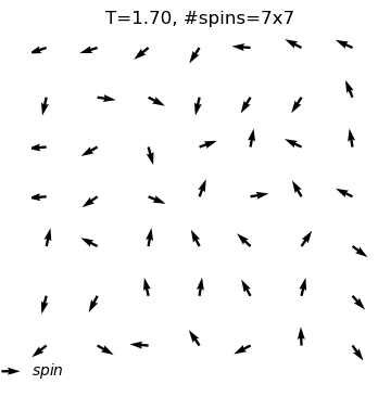
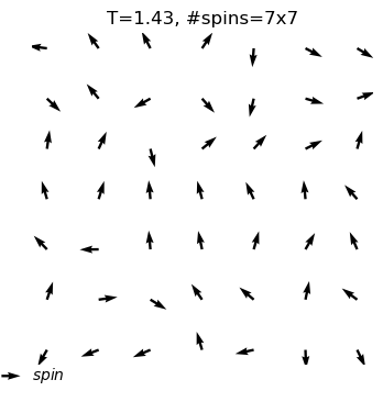
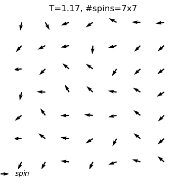
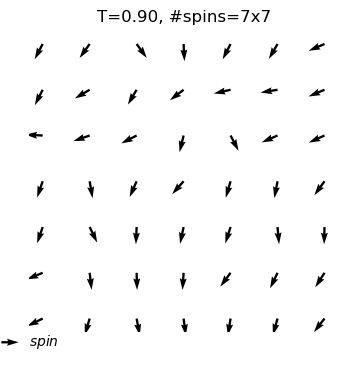
]]>Shiling Liang 梁师翎shiling.liang@epfl.chMonte Carlo Simulation of XY Model with Python2017-06-08T00:00:00-07:002017-06-08T00:00:00-07:00https://shiling42.github.io/posts/2017/06/XY-Model
A python program used for Monte Carlo simulation (Metropolis algorithm) of XY model.
What are the outputs?
equilibrium spin configuration in differnet temperature
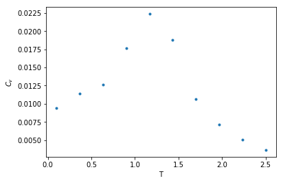
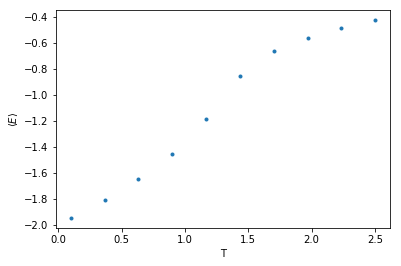
thermal quantities of XY spin system in different temperature
How to use this program
import the class
fromXY_modelimportXYSystem
creating an object as a X-Y spin system with given width and temperature
Use XYSystem(temperature = , width = ) to creat a class object. Two variables can be assigned to initilize the system: the temperature and the width.
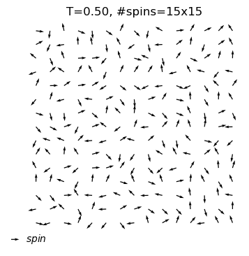
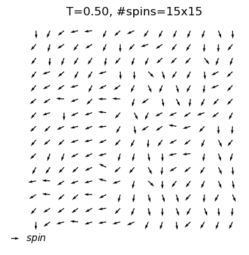
xy_system_1=XYSystem(temperature=0.5,width=15)
visulizingthe spin system
Using .show() to visulize the xy spin system as arrows on a two-dimensional plane.
xy_system_1.show()print('Energy per spin:%.3f'%xy_system_1.energy)
Energy per spin:0.056
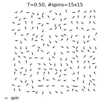
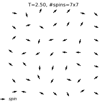
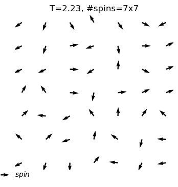
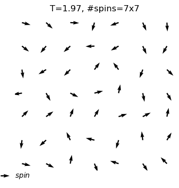
Now, let the system evolve to an equilibrium state
self.equilibrate(self,max_nsweeps=int(1e4),temperature=None,H=None,show = False) allows you to assign a new temperature, just simply do object.equilibrate(temperature = 3). If you want to keep the temperature defined before, leave it blank. And ·sohw=Ture` will let show the configuration of the system for each 1000 sweeps.