XY-MODEL
Monte Carlo simulation (Metropolis algorithm) on 2D XY-model
How to use this program
import the class
from XY_model import XYSystem
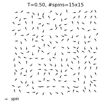
creating an object as a X-Y spin system with given width and temperature
Use XYSystem(temperature = , width = ) to creat a class object. Two variables can be assigned to initilize the system: the temperature and the width.
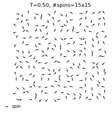
xy_system_1 = XYSystem(temperature = 0.5, width = 15)
visulizingthe spin system
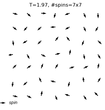
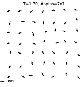
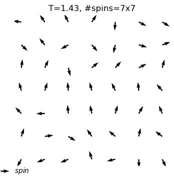
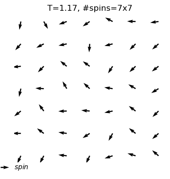
using .show() to visulize the xy spin system as arrows on two-dimensional plane.
xy_system_1.show()
print('Energy per spin:%.3f'%xy_system_1.energy)
Energy per spin:0.056
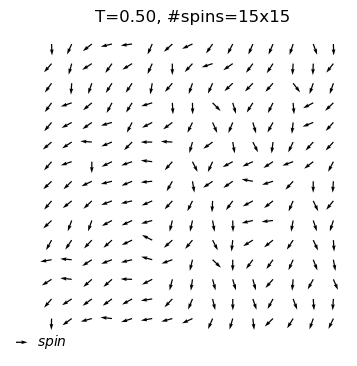
Now, let the system evolve to a equilibrium state
self.equilibrate(self,max_nsweeps=int(1e4),temperature=None,H=None,show = False)allows you to assign a new temperature, just simply do object.equilibrate(temperature = 3). If you want to keep the temperature defined before, leave it blank. And ·sohw=Ture` will let show the configuration of the system for each 1000 sweeps.
xy_system_1.equilibrate(show=True)
xy_system_1.show()
#sweeps=1
energy=-0.60
equilibrium state is reached at T=0.5
#sweep=504
energy=-1.72
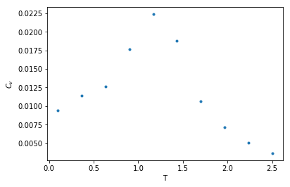
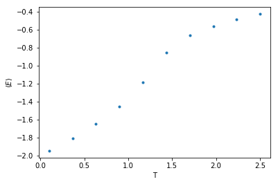
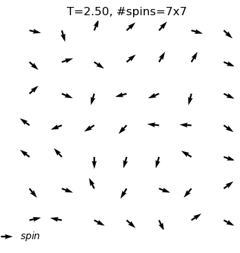
Observing the thermal quantities in different temperature - annealing approach
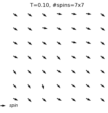
xy_system_2 = XYSystem(width=7)
cool_dat=xy_system_2.annealing(T_init=2.5,T_final=0.1,nsteps = 10,show_equi=True)
equilibrium state is reached at T=2.5
#sweep=6802
energy=-0.48
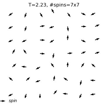
equilibrium state is reached at T=2.2
#sweep=3429
energy=-0.48
equilibrium state is reached at T=2.0
#sweep=9999
energy=-0.47
equilibrium state is reached at T=1.7
#sweep=2809
energy=-0.60
equilibrium state is reached at T=1.4
#sweep=989
energy=-0.74
equilibrium state is reached at T=1.2
#sweep=2253
energy=-1.35
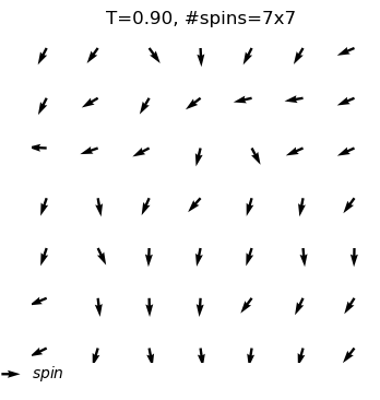
equilibrium state is reached at T=0.9
#sweep=636
energy=-1.68
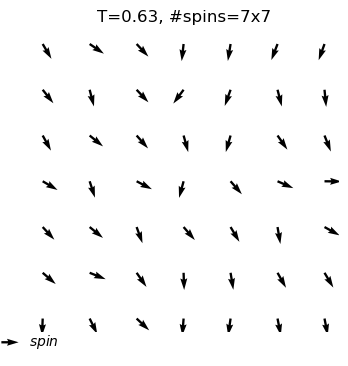
equilibrium state is reached at T=0.6
#sweep=837
energy=-1.72
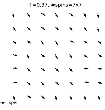
equilibrium state is reached at T=0.4
#sweep=548
energy=-1.86
equilibrium state is reached at T=0.1
#sweep=503
energy=-1.95